Wave Equations

One Dimensional Wave Equation
In Physics waves show up everywhere, therefore it is necessary that we develop a mathematical representation of these waves.  The most basic type of wave is the one dimensional traveling wave.  Imagine we have an equation of a wave that is a frozen snapshot.  We define some arbitrary point P that is on the wave and we will call this coordinate system the O coordinate system.  This wave has the very general expression..

If we allow the wave to move a certain amount of distance, the point P is now a distance of x=vt away from where it originally was.  The point P can now be described in either coordinate system as (x,y) or (x+vt,y).  Notice how the y component is the same in each system since this wave is moving horizontally.  We now express the function y in these new coordinates.

Where we have introduced a minus sign to take care of the situation when the wave moves in the opposite direction, and the notation x' to equal x+vt or x-vt.  Any function of this form represents a traveling wave, it need not be a sinusoidal function.  All the following examples represent traveling waves.

Our goal now is to set up a partial differential equation that describes a wave despite what y is actually equal to.
In this model, we are assuming constant velocity.

If we are talking about light, v=c which is the speed of light.  In order to see if a function is a traveling wave, you either try to look for x+vt or see if it satisfies this partial differential equation.

Harmonic Waves
A very important type of wave is a harmonic wave.  These type of waves are described either the sine or cosine function and have a periodic and endless nature to them.

Since the both of these functions are the same except shift a distance of pi/2 radians, we need only develop relations for one of them because the relation can immediately be applied to the other.  In this post, we will use the sine function.
Imagine you have a sine wave in the x,y plane.  This will be a snap shot of the wave so t is equal to a constant.  From peak to peak on the graph represents the wavelength of the wave (since the horizontal axis is spatial).  Wavelength is represented by the Greek letter lambda. If the wave moves a distance of lambda, then the same point can be described by shifting the x component a distance of lambda this type of movement is described also by adding 2pi in the sine argument. In other words..

We can now find an expression for k.

This is deemed the propagation constant and contains information about the wavelength.  The same logic from above can be done in the t,y plane with a constant position. The only difference is that the distance from peak to peak is no longer the wavelength.  Since the horizontal axis is time, this distance describes the period of the wave.

Combining these two expression we get a very familiar formula.

Where we have used the relation frequency=1/Period. Combining these first two expressions into the sine expression we come up with the general relation that is used for a wave.

Where we have deemed the expression 2pi*f equal to omega.  Omega is termed the angular frequency.  This is mainly because its units are inverse seconds and is simply done to make the expression for a wave look simpler.
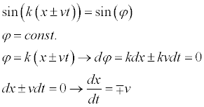
If x and t vary in a way such that the whole argument of the sine or cosine function is constant, it describes a situation of a plane wave, or wave front.  And we can see that..

This confirms that v represents the wave velocity.  Notice however the signs are flipped,  meaning the wave is moving in the positive direction then the expression x-vt is seen and vice versa.
Many times dues to initial conditions, we might not want to start looking at the wave directly from its "start" but rather shifted to the initial point of interest.  In these situations we simply add what is known as a "phase constant" to move the sine function to our interested starting point.

It is sometimes very useful to represent these wave equations in the complex plane. (See my post on complex numbers for more details.)  An expression that can either be the sine or cosine function is..

So depending on which trigonometric function we are using, we can either use the real or imaginary part of y. 

We now want to elaborate more no the notion of plane waves.  Firstly, we want a plane wave to describe a wave in all three coordinates, not just in the x direction.  For three dimensions, the wave equations looks like..

Note that k is now a vector, the k vector is pointing in the direction of propagation of the wave.  In complex form, the general expression for a wave is..

The partial differential equation associated with all three dimensions is..

Electromagnetic Waves

Electromagnetic waves have the same form as a sinusoidal wave.  In this case, the amplitude A represents the amplitude of either the electric or magnetic field.  Recall that light is simply the oscillation of electric and magnetic fields perpendicular to one another.

We start this section by showing Maxwell's Equations in free space in the differential form.

If we take the cross product of the third equation, and use the others during the derivation we obtain..

Note that the vector identity we used in the first step can be proved using the Levi-Cevita symbol.  If you do not know what this is, don't worry about it.  That particular proof isn't terribly important in this case. 

Notice that we ended up with a wave equation.  This is how light was deduced to be a wave.  We then related this expression to our earlier definition of a wave and found an expression to represent the speed of light.  A very similar proof can be done for the magnetic field by taking the curl of equation 4.

The energy density associated with the electric field and magnetic field in free space are..

The energy is therefore divided equally between the two fields, and the total energy density is given by..

We now consider the rate at which the electromagnetic wave delivers energy, or its power. In a certain time delta(t) the energy transported through a cross section of area A is the energy associated with the volume delta(V) of a rectangular volume of length c*delta(t), where c is the speed of light.  

We will now express the energy density u in terms of E and B.

When the power per unit area, is assigned the direction of propagation, it is called the Poynting vector.  The direction of propagation is equal to the cross product of the E and B fields. (Why?)

Since E and B are changing extremely rapidly, S is also changing very rapidly, not in direction however in magnitude. What we need to do now is take the time average of the amount of energy given by the Poynting vector.  This average is energy is called the irradiance.

Errors, and Statistical Theory

Why are errors so important in science? Whenever we make empirical measurements, it is impossible to make an exact measurement due to the limitations of the measuring device.  For example, if you were to measure a desk from top to bottom, and you use a measuring tape, you might find that the height of the desk is slightly over three and a half feet.  Meaning, the desk actually ends between the line of three and a half and three and 5/8 inches.  What then is the height of the desk?  You could "ball park it" and guess what the value could be, but a more scientific way of doing it would be to say the value is, not only in between these two marks on the ruler, but give the range in which it could be in.  In this case, you could say that the value is 3.5625 in (the number right between 1/2 and 5/8 of an inch) plus or minus an error amount.  How much is this error? In some cases it may be up to you, in others there are ways to calculate it.  In science you will be working with large amounts of date and the error equates to the standard deviation of the data.  For this particular example, a good number for the error would be plus or minus an eighth of an inch.  You could say 1/16, since it was between 1/2 and 1/8, it's up to you.  Keep in mind though, you never want to "over compensate" for the error.  An example of this would be saying the error is plus or minus an inch.  That's way too much!

As an example of the importance of errors, consider the following example.  Imagine we are measuring the temperature of a cooling object, and we get the two following readings..

Is the difference between these two temperatures significant?  There is no way of knowing without the error.  If the error is plus of minus 0.001, then the difference is most definitely significant. If however, the error happens to be 0.01, the error is insignificant.  When ever drawing conclusions or publishing work, all errors must be accounted for an documented, or else the data doesn't not mean much.

When working in science, it is important to distinguish the difference between the words, precise and accurate.  Precise means that all experimental values obtained, are all around the same value.  This value does NOT need to be the true value, (I will get to this a little later.) there may be some error associated with your device that is causing all the data to be shifted to an incorrect value.
Being accurate is actually obtaining close to the actual value of the experiment.  As an example, say you are measuring the speed of light, which happens to be 3 times 10 to the 8th.  (3E8) And you get values of 2.21E7, 2.23E7, 2.235E7, 2.36E7,...ect.  This values is very off from the actual value of the speed of light, one order of magnitude.  However, while this data may not be accurate, it is most definitely precise.  This is because all values obtained are close to each other.

This brings the next point of these notes.  The types of errors that can happen.  There are two types of errors that can happen to data.  Systematic error, and random error.  Systematic error has already been mentioned, it is the error associated with the system. (System---->Systematic)  This means that there is something flawed with the device that measures consistently incorrect.  In the previous example there was a systematic error of approximately 1.55E1 as all values were off from the actual speed of light by this amount.  The other type of error is called random error.  In this type of error, some random event happened that caused a data point to be way off the normal distribution of data points.  For example, say I wanted to start a stop watch right as someone dropped a ball to measure the time it took to hit the floor.  If I happened to sneeze right when he dropped it and didn't start it until the ball was almost touching the ground, this would account for a random error because for that one data point, the ball takes a LOT shorter time to hit the ground since I didn't start the watch until it was almost touching the ground and didn't have that much more left to travel.

When working with date points, the average value of them is extremely important.  The average value, or mean, is the sum of all the data points, divided by the amount of data points.  In other words...

Where we denote the average amount by a bar over the variable.  This notation will be used a lot.  While this is the most common way to get the average of a set of data, there is another way.  Say for example, that 50% of our measurements equaled 2, 20% of them equaled 4 and 30% equaled 6.  The average value is then..

Note that for the former case, this method is used when we have a distribution.  A distribution is essentially the percentage of each value of x there is for the entire set of data.  For a large amount of data, one could formulate a distribution function that shows a curve of the distribution of each value of x in the data.  If we were to sum all these distributions up over the x axis, we would obtain..

This is because distribution is percentage, and the sum of all the different amounts of percentages better be equal to 1, or we have made a mistake somewhere.  The limits negative to positive infinity are chosen purely for principles.  It represents the sum of all the data over all the values measured.  When we take the average over the distribution, we use a different notation other than the bar over the variable, we put angled brackets around the variable as well.  To obtain the average value of the distribution function, just as we did for the above example, we would multiply the distribution of each x value, by the x value itself and sum all these up.

The quantity f(x)dx actually represents the probability of the data.  So in our example of finding the average value, we said that the value of 2 occured 50% of the time.  Therefore, if you were to pick a value out of all of the valued obtained, there would be a 50% chance you get 2. If you sum these over an interval x-dx<x<x+dx, you obtain the probability of getting a value between  x-dx and x+dx.

So let's get back to errors.  An error in a measurement is defined as..

Where X is the true value or expected value.  When adding up errors or any data for that matter, it is helpful to use what is known as a root mean square of the data.  Notice that in the above expression for error, the error could be positive or negative depending on whether is is above of below X.  To get rid of this, we square the difference.  Squaring the difference also has another benefit, it better shows the difference between numbers. The difference between 7 and 8 is only 1, while the difference between 49 and 64 is 15! Much higher!  So the  method typically used is to square each difference up, then sum up all the squares, then take the square root and this will be the root mean square of the data.
So if we take the sum of the squares of the above errors and plug this value into the integral expression above for finding the average, we get what is essentially the average of the squared error.

The first term is what is known as the variance and is a measure of how far apart the values are from each other.  Note that a set of data can only have a variance if the data has an expected value.  Since the integral is measuring the error of each data point from the expected value, it is also inadvertently measuring the spread of each data point from each other.  Think about it, if all the data taken is EXTREMELY close to the expected value, the average of the squared errors will be smaller than if the values are further apart.  Therefore, if the value of the integral is small, the data points are closer together and if it is large, the data points are further apart.
The second term is simply taking the square root of the variance, completing the root mean square procedure.  This value is a measure of the spread of the distribution.  You could also look at this as being the root-mean-square of all the errors, giving an average error over the distribution.  This term is called the standard deviation of the data.

Imagine you measure 100 pieces of data for a given experiment.  The following day you measure another 100, and you continue to do this for a week.  At the end of the week, you have seven sets of data, each with 100 measurements.  If you wish to get the most accurate value for the true value of the data (X), then you would average each set of data, giving you seven averages, and then average all the averages together, giving you one average value that accounts for 700 measurements.  The standard deviation of this data will be denoted as sigma sub m.  What is the relation between the standard deviation of this average compared to the average of one set of data?  First consider a set of n measurements.  The error of each measurement is given by..

And the error in the mean of these data points is..

Some thought must go into why we were able to put X into the summation.  You really need to understand and treat the summation as the sum of n terms.  I know this may sound obvious but a lot of the time you can get locked into thinking of it as one item, when in fact it is n items. The average of the differences of each data point with the expected value, will be equal to the average of the data points, minus the expected value.  Think about it!
So the error of the mean, is the average of the individual errors.  This should make sense.  We now want to square both sides to further exemplify the error so it is more obvious.

Notice that the double sum went to zero.  Why is this the case? Think about it. E represents the error.  As you take more and more measurements, the value of the error gets really small.  The errors between e_i and e_j are independent and therefore their average is zero.

So we see that there are two ways of reducing the mean error and the mean standard deviation.  Either we take more and more measurements making n bigger, or make more precise measurements and make sigma smaller.  The latter is more cost effective than the former.

Treatment of Error in Functions
When we have a function Z=Z(A), the error in Z is given by..

This means we can write the relationship as...

As an example of how we would find the error delta Z, we use the following function..

For a function of more than one variable, the procedure somewhat similar..

As an example, if Z=A+B...

Least Squares Regression Line

Imagine you have a scatter plot of data points, and you want to find the best fit line to those points.  A technique you can use is called the method of least squares.  Our assumption in this derivation is that the error lies entirely on the y axis only.

For a given pair of values, the deviation of the i'th reading is...

The best values of m and c are taken when the following formula is a minimum.

The reason we are squaring each term is the same logic as the root-mean-square idea. (Mentioned earlier.)  To obtain the minimum of the above sum of the squares (Hence the term, least squares), you simply take the two partial derivatives, set them both equal to zero and solve.

Using this expression for m, and the second equation in our system of equations, one can find the best fit line of a set of data points.

Eigenvalue Problems and Diagonalization

The best way to describe this procedure is with an example. First we will solve the following eigenvalue problem..

This eigenvalue problem represents a transformation that transforms coordinate (x,y) into coordinate (x',y').  In the case of an eigenvalue problem, (x',y') is just a scalar multiple of (x,y). The next step in the diagonalizing process is to write the two sets of equations, substituting the eigenvalues.

Notice that we wrote the set of two equations as one matrix equation.  You can verify this by multiplying both sides out.  If you find the eigenvectors, you will find that.

Making t=1, and normalizing each vector we find that...

Plugging these value into the above matrix equation and assigning each matrix a name we get..

So we can see that the diagonal matrix resulting is a matrix with its eigenvalues down the main diagonal and zeros everywhere else.  The matrix D is the matrix which describes in the (x',y') system the same deformation that M describes in the (x,y) system.  As you can see the matrix is a lot simpler.  This means that the eigenvectors of the transformation matrix M give the best basis to use for the transformation.  The matrix C is some sort of transformation, whether it be a rotation, reflection or some sort of skewing.  Note however that, if C is not an orthogonal matrix, then the transformation will lead to a non-orthogonal basis of eigenvectors.

Let us now do an example.  Imagine we have two masses, and between them, they are connected by a spring.  Then imagine that on the other side of each mass, there is a spring that is attached to the wall.  (We are ignoring gravity.)
Since, these are spring we use the potential energy of a spring in the equation of motion for each mass...

Note that we assumed a few things.  We are assuming both masses are the same, and all spring constants are the same.  Also note that "y" in this case represents the displacement of the third spring. The displacement of the second spring is the displacement of the first spring plus the negative of the displacement of the second spring.  Thus x-y.  For this situation, we will assume the un-damped oscillatory motion.

So now we have an expression to find the eigen-frequencies of the system..

The eigenvalues and eigenvectors describe the possible motions of the system.  In the first case where x=-y, the two masses move in opposite directions, first the spring goes out like this <--- ---> Then like this
---><---.  (Use your imagination, those are arrows!)  In the second case where x=y, the two masses move like --->---> then like <---<---.  Note that the eigenvectors produced were orthogonal,  this is because we had a symmetric matrix!  Let us now move on to the system where the masses and spring constants are not equal.

Suppose we had masses and spring constants of, from left to right, 2k,2m,6k,3m,3k.  This problem is done pretty much exactly as the previous one..

Note how we didn't need to actually solve for the constant vectors a and b since we know this will be a solution and it isn't needed to find the eigenvectors.  The behavior of the eigenvectors this time is the same as last time except in the case where the masses oscillate in opposite directions, one has 3/2 the magnitude of the other.  Note that since the matrix wasn't symmetric, the eigenvalues were not orthogonal! This could easily be fixed by a change of variables in the matrix or normalizing the existing vectors, but all we care about is the direction so there is no need.

As a final problem to this post, we will model a tri-atomic linear molecule with the two end masses of mass "m" and the middle molecule with mass "M."  We will model the forces holding them together as springs, so it will be very similar to the two previous problems.

So the first possible motion is all the masses moving to the right together, as in translation.  The second motion is when the middle mass stays stationary and the two side masses oscillate in opposite directions.  The third motion is both side masses oscillate in the same direction as the middle mass oscillates in the opposite direction with magnitude 2m/M.
1. m--->M-->m--->
2. m--->M<---m
3. m---><---Mm--->

Designing an Achromatic Doublet

The goal here is to develop a quantitative approach in designing an achromatic doublet that reduces chromatic aberrations.  We will have two lenses cemented together, the choice of lenses is up to you but lets keep it general.  The refractive power of each lens, by the lens-maker equation is..

We relate the lens to the Fraunhofer lines. The Fraunhofer lines are the dark lines in the emission spectrum of the sun, or the colored lines in the absorption spectrum. The refractive index of a material is actually not constant, but is a function of wavelength.  When we say the refractive index of glass for example, is 1.50 this is an average value of the index over the visible spectrum.  We use the Fraunhofer lines as a industry standard.  Light is shined through an element and certain absorption spectrums are produced.  When we are finished with the mathematical model, we test it at the broad ends of the spectrum and calculate the chromatic aberrations to see how good of a lens it is.

First thing we need to do is find the sum of the refractive power of the combined lens doublet.  This is simply the sum of the individual refractive powers if there is no space between them. (Since this is a doublet, there is no space between the lenses.)  Combining this idea with the former expressions...

We want the refractive power to be independent of wavelength, therefore the derivative of P with respect to wavelength should be equal to zero.

The partial derivative of the refractive index can be approximated using the F and C line of the Fraunhofer wavelength for the given material.

We now essentially want to expand the above expression to include the dispersion constants for the glasses used.  We then define a constant "V" which is defined as the reciprocal of the dispersive power.

From this, we can use the properties of the lens to find all four values of the radii!