A mind dump of mathematics...

Normally I use this blog to post things that I am currently studying. But recently I have discovered that my blog is receiving a good amount of page views via google. So I from time to time I will be posting things that I feel as though people may need help with.

One such topic that came to mind is integrating using trigonometric substitution. Over the years I have seen this topic taught by many professors and I have yet to see a way that I have liked, they all used methods of memorization instead of methods of logic. (I don't like to memorize things! It is much easier to remember the logic than formulas!)

I will present an easy to remember method of how to do trigonometric substitution. So, lets start out with an example..

The trick to these integrals is to relate it to a triangle. If we look at the Pythagorean theorem, we can put it in the form identical to the form in the denominator.

Thus, we know that the hypotenuse to our triangle (the variable c) is equal to x, and a=1. So let us construct the triangle from this!

NOTE: The choice of which leg to put "1" is completely up to you. Since both "a" and "b" in the Pythagorean theorem can both be legs, it does not matter where you put it. It will only change your substitution, not your answer.

So from this we see that..

Now that we have these relationships, lets plug it into our integral.

And that's all there is to it! It all boils down to simply relating the radical term to a triangle using the Pythagorean Theorem. You MUST remember to substitute for dx! A common beginner mistake is to forget about dx! You need to find dx by first establishing x, then differentiating it! Let's do a couple more examples.

So a "tip off" that we need to use trig-sub is seeing the radical term. We once again relate this to a triangle. The radical is of the same form as the previous example so we know the hypotenuse must be 3 and one of the legs must be sqrt(5)*x

We can now draw some relationships from this and substitute into the integral.

Let's do one more "typical" example then we will use this for something more exotic. For this one I will do much less explaining.

We now relate this to the Pythagorean theorem.

We see from the Pythagorean theorem that one leg of the triangle is equal to 3 and the other leg is equal to x. (The choice of which leg goes where is up to you!)

For this last example, I will show you that you can use this technique in more places than just square roots. This is something that I actually did at one point. I couldn't remember the integral of 2^x and I didn't have anywhere to look it up. (Before I had a smart phone!) So I did this to figure it out.

We can construct a triangle from this. It need not be in the Pythagorean form. You can do it in the following way.

From this we can draw trigonometric relations..

Pretty awesome!!

Conclusion:

These examples were some basic trig-sub examples. They can get more complicated, as in having "x's" in the numerator as well. But just approach them in the exact same manner and they should turn out okay!

(The following are my notes from "Quantum Physics" Chapter 5 and 6 from Stephen Gasiorowicz)

The Hamiltonian Operator:

The time dependence of the wave function is given by..

On the right side of the equation, the wave function is acted upon by the Hamiltonian Operator, it is an operator version of the total energy.

Where from here on out, we will represent operator with hats over them.

If the potential function has no time dependence, then the Schrodinger equation becomes separable and we get a relation for the function that describes the position. The solution is..

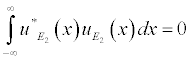
Where E are the eigenvalues and u_E(x) are the eigenfunctions of the wave function. Eigenfunctions that correspond to different eigenvalues are orthogonal, namely..

The eigenfunctions of H form a complete set, namely for any arbitrary square integrable function of x, one that satisfies the following..

may be expanded in terms of the eigenfunctions of H, so that...

Namely, we can write the wave function as a linear combination of its eigenfunctions.
These eigenfunctions can be multiplied by a constant to become normalized so the sum over all x of the same eigenfunction is equal to 1. (Because remember, this represents a probability!) If the eigenfunctions are different, the sum over all x will equal zero because as stated, they are orthogonal to each other. So it follows this condition..

Where we have used the kronecker delta function.
Since we have stated that the position wave function can be written as a linear combination of its eigenfunctions, the entire wave function, one that depends on both space and time, can be written as..

Energy is just one observable of a system, we also have momentum. We recall (from a previous post of mine) that the momentum eigenfunctions are described by the following differential equation.

The momentum operator, like the Hamiltonian operator has real eigenvalues. This is because it is a physically observable quantity. Any operators with real eigenvalues only are called hermitian operators.

The Interpretation of the Expansion Coefficients:

From previous posts, at this point we know that...

Directly from the book, pg 97

1. The results of any given measurement can only be one of the eigenvalues.

2. The probability that the eigenvalue will be found, or, equivalently, the fraction of systems in the collection that will be found to have the eigenvalue a, is |C_a|^2.

3. After a measurement on a member of the collection yields a given eigenvalue a_1, for example, then that particular system in the collection must be projected by the measurement into the state u_(a_1)(x). Only in this way can we be sure that an immediate repetition of the measurement of the observable A gives the same result.

The value of the observable A for a system has any one of the eigenvalues is unity. This means..

We can use this to prove an identity used in Fourier Transforms.
We know that...

We will now define a Hermitian conjugate operator denoted Q^+

For hermitian operators, we know that the expectation values must be real, so..

For any two operators A and B...

Degeneracy and Simultaneous Observables:

We will now discuss the condition for when the same eigenfunctions apply two operators.

The eigenfunctions u_a(x) corresponding to the operator A,

will be simultaneous eigenfunctions of another operator B when..

This implies that..

For one eigenfunction, this isn't very interesting, but if we were to sum this over all eigenfunctions..

So the condition for the same set of eigenfunctions to apply to both operators is, the operators must commute. (Remember, the above notation indicated the commutator of two operators.)

Does the converse apply? If we have two hermitian operators, and they commute, does it necessarily mean that we will have the same set of eigenfunctions?
Under these circumstances..

So the function Bu_a(x) is also an eigenfunction of A eith eigenvalue a. If there is only one eigenfunction of A that corresponds to the eigenvalue a, then we must conclude that Bu_a(x) is proportional to u_a(x). We write this proportionallity as..

We can therefore conclude that u_a(x) is simultaneously an eigenfunction of both A and B. We should therefore change the notation a little.

But what about the case when we have degeneracy? Namely, when we get more than one eigenfunction from one eigenvalue. So we have..

For these circumstances, all we can do is say that when B acts on either one of these eigenfunctions, it produces a linear combination of both of them.

This isn't a problem, we will simply choose a linear combination (that we will call v) such that...

Bra-Ket Notation (Dirac Notation):

(To anyone who may be reading these notes, this will not be an in depth look into Bra-Ket notation as I am already aware on how they work, I use this website for my notes and it would take too much of my study time to go into something that I already know a great deal about. I do this sometimes, but as of right now, time is of the essence!)

For the following relation,

The notation on the left hand side of the equal sign is called the Bra-Ket notation. (Get it? Bracket?) The term with Phi in it is the Bra vector and the term with Psi is the Ket vector. For every ket there is a bra that is simply the complex conjugate of the ket function. So since Phi is in a bra form, its notation in the integral must be the complex conjugate. These vectors describe a state.

When an operator acts on a state it creates another state. We write this in the following way.

Where the left hand side represents the operator acting on the ket vector and the right hand side is simply a way of writing the resulting vector.

Another example of Dirac notation is..

Recall our definition of the Hermitian conjugate operator.

We will now examine the expansion theorem using this notation.

From the expansion theorem, a wave function can be written as..

We will now do the example in on page 109.

Show that the eigenkets of any hermitian operator are orthogonal to each other if the eigenvalues are different.

The eigenvalue equations read..

Thus the eigenkets are orthogonal to each other then their eigenvalues aren't equal to each other.

Suppose we ask: What is the probability that if we make a measurement of the position of the state represented by |psi>, we find the value x?
Since the position is an observable quantity, we can pretty much assume that it is a Hermitian operator. We will denote this operator as X. This operator will have a complete set of eigenkets, whose eigenvalues are the numbers x.

Using the expansion theorem, we can write..

We write this as an integral because x represents a continuous eigenvalue.
Using the orthonormallity of the eigenstates in the form..

We can calculate C(x') by multiplying the integral equation above by the x' bra vector.

The magnitude of the expansion constants |C(x')|^2 is the probability that a measurement of the position of the state |psi> yields the value x. This is precisely the definition of |psi(x)|^2! So all we have to do is replace C with psi and change around the notation..

Similarly, we could show that the momentum space wave function for the state |psi> is..

We can now make several points:
The completeness relation in terms of the position eigenkets reads..

The unit operator can now be inserted at will, for example..

Consider..

Projection Operators:

We will not return to the interpretation of the expansion coefficients we developed earlier. For simplicity, we will deal with discrete eigenvalues.

P is the projection operator because it has the property that when acting on an arbitrary state, it projects it into a state of |n>, with probability amplitude <n|psi>. What we have shown above is that if we use the projection operator again, after first using it once then it changes nothing. This is because when we take a measurement we force the system (using the projection operator) into one of its eigenstates. Further measurement will only yield the same result, as it should.

If we were to write the average energy...

So we can write the operator H in terms of its eigenvalues and corresponding projectors.

The Energy Spectrum of the Harmonic Oscillator:

We first start by writing the Hamiltonian for the Harmonic Oscillator.

We introduce a special notation for the operators in the terms H -1/2(hbar)w is factored. (With an extra factor of 1/(sqrt(hbar)) to make them dimensionless.

Thus A|E> is also an eigenstate of H, but with energy lowered by (h-bar)w. Is we apply A- again to the state A|E> we again get another energy lowering. This lowering can only go as far as the ground state. (The lowest energy level.) We denote the ground state as |0>. Because of this, we must write that A|0>=0. Thus the ground state energy is..

It can be shown in the same manner that the A+ operator raises the energy level by 1.

The thing about these operator is that it does not keep the state normalized. We must therefore construct a normalization constant.

We see that A acting on any polynomial f(A+)|0> is equivalent to d/dA+ acting on that state. Let us now consider <0|A^m(A+)^n|0>. This goes to zero unless m=n so we end up with..