Motion of a Particle in one Dimension

This post is taken in reference to the book "Mechanics: Third Edition" by Symon
The motion of a particle is governed by Newtons Second Law, namely..

Recall that the definition of momentum is..

Combining these two expressions we simply get Newtons Second Law in another form.

Solving for "dp" and integrating we get the integrated form of the momentum theorem.

The integral on the right hand side is the force over the time interval, namely the "impulse."

Recall that the definition of kinetic energy is..

Let us now take newtons second law in terms of velocity (from the very first equation) and multiply both sides by "v."

So as you can see, we end up with the work kinetic energy theorem!

Starting out with the integral form of the change in momentum we can obtain a function that describes the velocity and hence, the position after integrating.

As an example of seeing these equations in action, imagine we have an electron.  This electron is about to be acted upon by an electric field given by the equation..

Recall that the forces acting on an electron is..

Using Newtons Second law as we previously did, the equation of motion is..(We will use the initial conditions t0=0 and x0=0)

We now investigate the case where the force applied depends on velocity alone.  This type of thing comes up a lot when dealing with drag forces such as wind resistance or friction.  In such a case, Newtons Second Law looks like..

Since the force is in terms of velocity, we want the "dv" to be with the F(v) as to make integration easier.

The integral can be solved in principle, and assuming we can solve for "v" then we could integrate form there and obtain position.

Often times, frictional forces are proportional to a non-changing power of velocity with a proportionality constant.

Where the sign is chosen to oppose the motion of the object.  Often times n=1 or 2.  In this next example we shall take n to equal 1.  If we are driving a car and all of a sudden the car turns off, and we are coasting, there is no more force propelling the car and the only force acting on the car is the frictional force. (Lets assume that the only one frictional force is acting on a car and it takes into account both the tires friction on the road, and the wind resistance.  This force will be equal to "F(v)=-bv."  Plugging this into newtons second law.. (Taking the initial time to be equal to zero.)

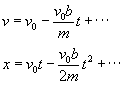
Notice that the velocity of the car never mathematically stops, it just gets smaller and smaller.  However, the position IS finite, if we take the limit we get..

The velocity goes against intuition as we know the car does indeed come to a stop eventually.  To solve this delema, all you would need to do is define a velocity that constitutes the boat as being stopped, and then just solve for "t" and find the stopping time.  What is interesting, is if you write out the first couple terms in the Taylor expansion, it is the equations of motion of a particle acted upon by a constant force!

When the force acting on a particle depends only on the position, (also known as a conservative force) by the work kinetic energy theorem.

We must not define the potential energy to be the work to go from point "x" to some standard point "x_s."

Now we carry out the integral for work using the definition for potential energy..

Thus we have, the conservation of energy equation!

We know that the sum of the initial kinetic and potential values will equal to total energy in the system.  If we express this value as "E" and then solve for velocity in the expression for kinetic energy..

If we wish to find "x", it can be found by solving for it after we do a little rearranging and integrating..

Because of our definition of potential Energy, we can now define the force in terms of the potential energy.  I mentioned before about having a standard point x_s, when changing this point, you are essentially adding a constant to V.  Since the derivative of V is the quantity that enters systems, this constant means nothing, there fore you can always call the initial point x=0 because we need only be concerned with the change in potential energy from the two points.

As an example, lets analyze a mass attached to a spring.  We know from hookes law the restoring force of the spring will be F=-kx.

Using K+V=E, we obtain...(Using initial x and t as zero.)

Now use a trigonometric substitution to evaluate the integral.

Thus, the position oscillates back and forth as expected to come from a spring.

If we have a mass attached to a spring that is oscillating back and fourth with no frictional forces, the equation of motion from Newtons Second Law is..

The solution of this equation is that of a simple harmonic oscillator, of the same type we just derived using energy methods.  If however, we add a frictional component to the spring, we have what is called a damped oscillator.  Meaning that it slowly comes to a rest as time goes up.  This is a more realistic situation.  

Frictional force is often modeled as being directly proportional to the velocity of the particle.  This should make sense as the faster you go, the more air resistance acts on you.  It is typically drag_force=bv, where b is a proportionality constant and v is velocity.   Plugging this into Newtons Second Law, the equation of motion now becomes..

This is a second order homogeneous ordinary differential equation with constant coefficients.  If there is a force acting upon the spring mass system, then the right hand side would simply be equal to the force F(t).  So in the process of solving this differential equation we get a quadratic  algebraic equation.  Solving this we get..

Is this the final equation?  No it is not simply because there are a few condition we must take into account.  One condition is that gamma squared is larger than omega squared, another condition is the opposite. And the last condition is that they are equal.  We will now go over each case.

Beginning with the second case where omega squared is larger than gamma squared, we get a complex solution.

Lets begin by making one more definition, we will define a second frequency as..

We now do the following work..

It is easy to see from this solution that the mass spring system is oscillating with a frequency of omega_1.

We now consider the condition in which the mass spring system is over damped, in other words, the drag coefficient b is large enough to cause the square root term to be real and the system to act differently.  The solution is simply.. 

We now know that the terms in the exponent are real.  Both terms in this expression decrease exponentially.  One term is faster than the other however. (Why?) So as you can see, the systems position decreases exponentially and does not oscillate.  This is exactly what we would expect from an over damped system such as the mass spring system in a very viscous liquid.  Certainly it is not hard to imagine that there will be no oscillations in this case.

For the third case, we have yet another damping, except this one approaches equilibrium at a much more desired rate known as the critical damping.

Where this solution is obtained by using the variation of parameters on the single solution to the differential equation to obtain the second solution.

We now move onto the topic of the forces oscillator.  I briefly mentioned this type of oscillator earlier.  In a forced oscillator situation, the right hand side of the equation of motion is no longer zero it is F(t).  The most important case for a forced oscillator is a sinusoidal force, or simply put, an oscillating force.  This would be in the form..

Where theta specifies the phase of the applied force. We will now use the method of undetermined coefficients to solve this differential equation.  Our guess for the solution will be trigonometric as is the right hand side.  We could guess that the solution will be the sum of a sine and cosine term and solve for the coefficients, and that would work just fine but it is easier to write everything in terms of a complex number and assume x is a complex solution, and then just take the real part out of it.

We can be expressed into polar form. (See one of my previous post about complex numbers.) (Bold number will represent their complex counterpart.)

Now we can take the real part from this and obtain our answer.  The real position and velocity are..

Therefore the general solution to the equation of motion is...

Where A and theta are the two arbitrary constants and must be found from initial conditions.  The first term is the transient term and dies out as time progresses and the second term is the steady state and describes the motion after the initial start of the mass spring system.

Sometimes the definition for beta is different to make the final answer analogous with other models in electrical engineering and also to make it so all the terms in the exponent have no minuses.  The work for this is the following..

We now move onto the final topic of this post, and that is a forced oscillator with multiple forces acting upon it.  This type of problem is solved in the very same way.  All one must do is solve the system for each force individually and superimpose the solutions. A particular example is when F(t) is the sum of multiple sinusoidal forces.  In this case (and any case with any super imposed forces) we have already solved the differential equation, we just need to plug in the force into F(t). (Note that we are only plugging in the amplitudes!  This is because F_0 was in the solution, not F(t)!)

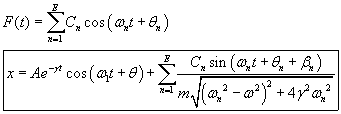
This is the general solution.

Complex Numbers

A complex number is simply a number "z" in which there is a real part and an imaginary part. "z = a +bi" is a complex number with real part "a" and imaginary part "bi."  Note that "a" and "b" are both real numbers!  One useful aspect comes from plotting these complex numbers in what is known as the "complex plane."  The complex plane is exactly the same as the ordinary Cartesian plane except what is plotted isn't x and y, but rather real vs imaginary.  (Real being on the x axis and imaginary being on the y axis)

Plotting the number z on the complex plane, we simply go "a" units on the real axis and "b" units on the imaginary axis.  (Note that you are plotting b, not ib!)  If you connect a line from the origin from this point you now have a line segment (labeled "r") originating from the origin to the point (a,b).  Using trigonometry (taking the angle to be from the horizontal) you will find that..

Where we have used Euler's formula to replace the trigonometric terms with an exponential term.
Therefore, there are two ways to write a complex number, we can write it as a+bi or in its polar exponential form just shown.

A notation that is useful is the Re(z) and Im(z) notation.  Re(z) simply means the real values of the number z, and Im(z) simply means the imaginary values of the number z.  For example, if we had z = 1+2i.  Re(z)=1 and Im(z)=2 (Not 2i!!).

A term that you must know is known as the "modulus" or "norm" of z.  Its notation is that of the absolute value notation and is defined as the length of r in the complex plane.

Where the last term is the square root of z times z bar.  The term z bar is the conjugate of z.  (For those that don't know, the conjugate of any complex number a+bi is a-bi).  A useful relation to the conjugate of z is..

For an example, if we wanted to write the number z = -1-i in polar form, a=-1 and b=-1.  Just like in trigonometry, the angle can take of infinite values. (Because you can simply go around the whole circle and you would be in the same place, yet have a bigger angle value.)  The general formula for the angle in this case is..

Notice that we did not use the value of pi/4 as the answer! This is because the actual point is in the third quadrant and pi/4 is in the first! So we must exclude all angles in the first quadrant in this case because that is not where the point is located.  For simplicity, take n=0.

Complex numbers can also come up in equations.  These are known as (not surprisingly) complex equations.  This is best explained with an example.  Say we want to find the values of x and y in the equation..

All we need to do is expand and equate the real parts on the left with the real parts on the right, and the same for both the imaginary parts.

You may be asking yourself, "Since we have graphed a point using a complex number, does that mean we can have graphs of complex numbers?" The answer is yes!  The way it works is basically exactly how polar graphs work.  The only difference is replacing "r" in the polar graphs with modulus of z, or |z|.  So |z|=3 is a circle of radius 3 in the complex plane.

Next on the agenda is complex infinite series! A complex series in general looks like this..

The conditions for convergence for a complex series is...

So basically, both real parts must converge for the series as a whole to converge.  This makes a lot of sense! Typically you only need to split the series up into its components if the standard ratio test fails to show convergence.  As an example lets test the following series for convergence.

This next example is an example where the ratio test fails and we must write out the first couple of terms to find the real and imaginary part of the summation.  We must then find the convergence of these parts.

As you recall from your Calculus courses, you often needed to find the range in which an infinite series converges.  This was called the radius of convergence.  We will now be looking into the power series..

As an example let us find the convergence of the following series using the ratio test..

So what does this mean?  This means we have a disk of convergence.  Recall that previously I mentioned that |z| acts as r in polar coordinates.  So the disk of convergence is a disk of radius 1.  An interesting thing to note is that the real axis length of the disk is 1, this is the radius (of the disk!) of convergence of the real part of this series! That is the very reason it is called the radius of convergence!

We can use the exponential definition of a complex number to come up with a useful relationship.

This relationship can be used to find the formulas for cos(nt) or sin(nt)! (I am using "t" as theta)  As an example, let us find the equation for finding the cosine of 3 times theta, or cos(3t).

 Very cool!!

The function e^z can be written as a complex infinite series, but another way to write it is as such.

This notation is usually used to find exact values for e^z for a given x and y. (Note that I have replaced a and b with x any y, that shouldn't be a problem! They are just dummy variables!)  If you have e^z and e^(-z)  and set z equal to just its imaginary part "i" times theta, this creates a system of equations in which you can solve for sine and cosine.

These formulas are good to use in integration since products of exponents are far easier to integrate than products of trigonometric functions.  These formulas also work for any value of theta, even complex values!

If we use the above formulas to with a complex value of theta "z" we can get a couple of very useful formulas! Firstly, theta will only have an imaginary part such as "iy".

These come up so often in problems that they actually have their own name, the hyperbolic functions.  Notice that the "i" is not included in the hyperbolic sine function.  These pretty much follow all the rules for the normal trigonometric functions as they should since the hyperbolic functions are simply the imaginary components of the sine and cosine function!

Our next objective is to see if we can find the logarithm of a complex number.  Namely..

So a complex number has infinitely many logarithms! (Since every theta has an infinite amount of other thetas that are equivalent. 

And that's my sch-peal on complex numbers!